Triangle Subdivisions
– Jan. 30, 2021
This article showcases a family of triangle subdivisions, where very little mathematics is involved. Every triangle will be subdivided into exactly two new triangles at every step, in one of the easiest ways possible. The subdivision is complete, meaning that after every iteration of subdivision, the area of all resulting triangles equals the area of the triangles from the previous iteration. There are no gaps created (like in the Sierpinsky triangle), and the subdivision will always stay exactly within the bounds of the previous triangle.
An easy way to subdivide a triangle into two new triangles is to draw a straight line from one of the corner points (vertices) to a point on the opposite edge.
There are always three triangle vertices to choose from. The point on the opposite edge can be anywhere, but the most straightforward choice with an easy calculation is to take the midpoint of the opposite edge. Taking the midpoint also results in some beautiful symmetries.

For an equilateral triangle, all three possible subdivisions are equal (but rotated by a third of a full rotation as seen on the image above). The new triangles are always two right triangles. The image below shows the three different subdivisions for this right triangle.
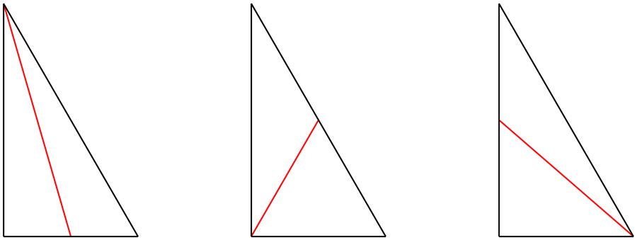
As you can see, all three subdivisions result in different triangles. Note that for the result in the center, one new triangle is an equilateral triangle, and the other triangle is an isosceles triangle.
By the nature of this subdivision, every right triangle subdivides into two isosceles triangles when the right angle is chosen. Both of those isosceles triangles can subdivide into 2 of the original right triangles.
In the example above, one of the isosceles triangles was an equilateral triangle, which is only the case if the original right triangle has 30° and 60° angles.
Below are the three subdivisions for the isosceles triangle.
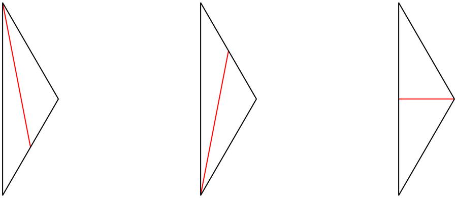
The first two outcomes are the same, but mirrored (which is expected since an isosceles triangle has two equal sides and two equal angles). For the third one the result is two right triangles (the same 30°–60°–90° triangle as before).
This means that there could be repeating patterns in the subdivision. For example:
Equilateral triangle → right triangle → equilateral triangle.
Right triangle → isosceles triangle → Right triangle (always the same one as 2 steps before).
When the same angle keeps getting subdivided, the resulting triangles will get sharper and sharper.

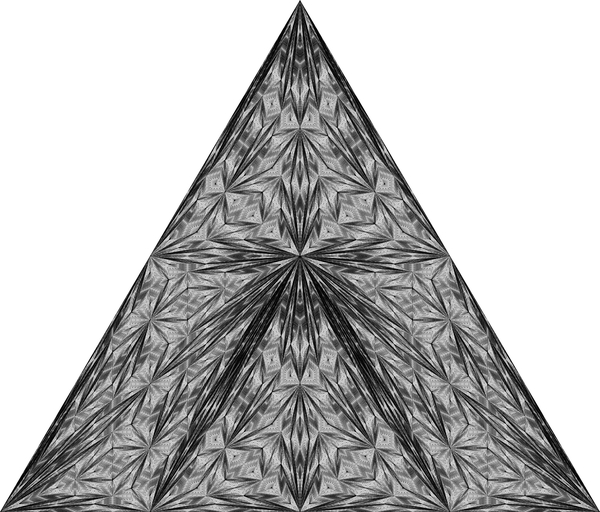
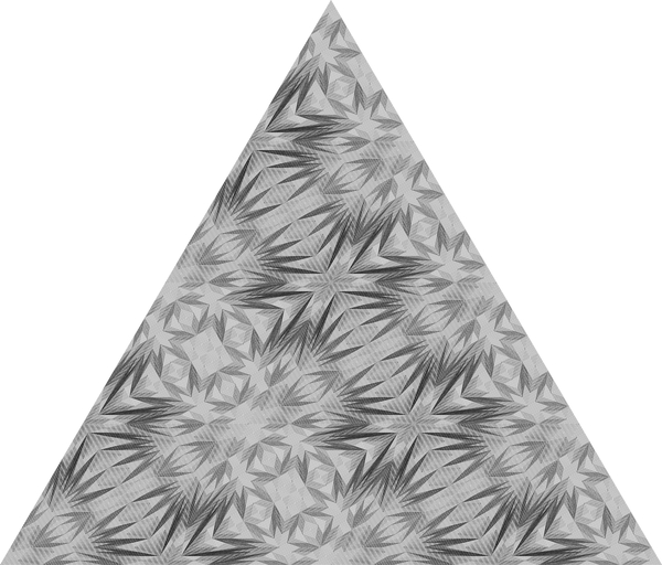
Alternating between different vertices produces more interesting images. Below are two examples with 20 iterations. There are over 1 million triangles drawn, but the image was resized, so the individual triangles are not visible any more.
How many unique variations are there?
For every number of iterations, we can calculate the number of variations.
For 0 iterations it is is the original triangle only.
For 1 iteration, there are 3 different subdivisions.
For the 2nd iteration, each of those 3 previous variations can be subdivided in 9 different ways because every variation from iteration 1 consists of 2 triangles. Each of those 2 triangles can be subdivided in 3 different ways, which results in 32 new variations (for every variation from iteration 1).
In the image below, you can see the 3 different variations from the 1st iteration on the first line.
Below them are all 9 variations in blocks of 3 x 3.
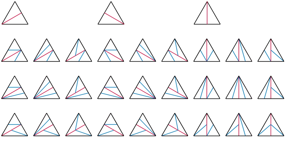
Use the toggle button to switch between equilateral triangles, and right triangles with 3 different side lengths.
The subdivisions are exactly the same, but the original triangles are different.
If rotation is allowed, we can see that only one third of the 27 equilateral triangles are different.
For the right triangle every subdivision is different, because this triangle has 3 different side lengths, and rotation will not result in an equal image.
If reflections are allowed, the number of unique subdivisions shrinks even more for the equilateral triangles.
In the image below are the equilateral triangles re grouped. From now on, I choose to only work with the rotation where the first subdivision (red line) is a vertical line, because that one is the most intuitive when talking about reflections.
On the first line are the six unique ones.
The 3 triangles on the second row, are equivalent to the triangle above it, when reflecting through the red line, which is the division line from the 1st iteration.

The first three are symmetric by reflecting trough the red line.
Note that this grouping for the equilateral triangles is visible in figure 7. Take one of the 3 by 3 groups of triangles, and notice the diagonal with symmetric variations from top left to bottom right. For each of the resulting 6 triangles, you can find the other half of the pair on the other side of the diagonal.
The number of triangles per iteration is doubled at every step, since we divide every triangle into exactly two new triangles. Let's call the number of triangles T, and T(n) = 2n.
V is the total number of variations, when no rotations and reflections are taken into account.
V is a multiple of the number of variations from the previous iteration, because for every single previous variation, a number of new variation can be made
(look at figure 7 to see that there are 9 new variations for each of the 3 previous ones).
This multiplication number is 3T(n-1), where T(n-1) is the number of triangles from the previous generation, since for every triangle from the previous iteration, 3 new subdivisions can be made.
The number of triangles in the previous iteration is 2n - 1.
So V(n) = 32(n - 1) * V(n -1).
Since we know that V(0) = 1, we can fill it in and calculate V(1), V(2) etc. I find that V(n) = 3(2n - 1).
Note that this is 3 to the power Mersenne number(n).
| Iterations | Triangles (T) | V | S | U |
|---|---|---|---|---|
| 0 | 1 | 1 | 1 | 1 |
| 1 | 2 | 3 | 1 | 1 |
| 2 | 4 | 27 | 3 | 6 |
| 3 | 8 | 2187 | 27 | 378 |
| 4 | 16 | 14348907 | 2187 | 2392578 |
| .. | ||||
| n | 2n | 3(2n- 1) | V(n - 1) | (S2 + S) / 2 |
Now I like to consider the equilateral triangle subdivisions only, and look at the unique and symmetrical subdivisions. I listed them in the table above as U and S respectively. As we have seen before, there are 3 rotations for every variation, so we only have to consider 1 / 3th of the total variations (32n-2, subtract 1 from the powers of 3.). This 1 / 3th of the total is always a square number (it can be rewritten as (32(n-1)-1)2). They can be listed in a square grid (equal number of items per row as per column), like I did before in figure 7 for all 3 rotations. For every variation, there is an equivalent one, reflected through the red line (subdivision line from iteration 1), except for the symmetrical variations (they stay the same after this reflection).
When you open the file in this link, you can see the same idea for one third of all 3th iteration subdivisions, in a 27 x 27 grid.
On the diagonal you will find 27 symmetrical subdivisions, and every single subdivision on one side of the diagonal has a reflected version on the other side of the diagonal.
The number of symmetrical subdivision (the diagonal) is the same as the number of rows or columns in this grid. It is the square root of 1 / 3th of the total variations.
This turns out to equal V(n - 1). This number of symmetrical subdivisions is called S in the table.
This means that the total variations V(n) can also be expressed as 3 * (V(n-1))2.

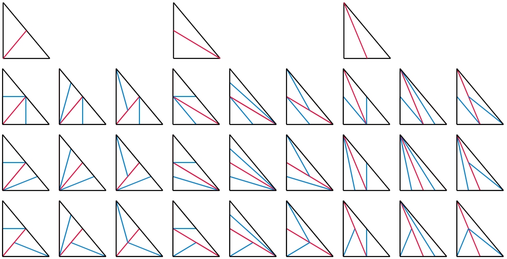
All 27 symmetrical subdivisions after 3 iterations are listed in the image above.
Note that the vertical red line is the division line from iteration 1, the two blue lines are the subdivision lines from iteration 2,
and the 4 green lines are the subdivision lines from iteration 3.
For each of the 3 symmetrical variations from iteration 2, 9 new variations could be constructed.
Although the previous iteration had 4 triangles, only half of them (one side of the red line) are relevant to achieve the symmetrical results.
Those two triangles could be subdivided in 32=9 different ways. For the next iteration I expect 27 * 34 symmetrical variations.
In general S(n) = S(n - 1) * 3T(n - 1) / 2 = S(n - 1) * 3n - 2 (for n > 1 and S(0) = S(1) = 1).
This turns out to be S(n) = 32(n - 1) - 1 for n > 0 and S(0) = 1.
The total number of unique variations is all the symmetrical ones on the diagonal plus one half of the remaining variations.
Since S is the number of items on the diagonal but also equals the width and height of the variations, the number of unique variations can be expressed as (S * S) / 2 + (S / 2).
S * S equals all variations in the grid. When we take half of it, we have to add the remaining half of the diagonal (S / 2).
So U(n) = (S(n)2 + S(n)) / 2.
I also uploaded a file with all 2187 unique symmetrical 4th iteration subdivisions here (it is ~28mb and 7050 x 7050 pixels).
Defining subdivision strategies
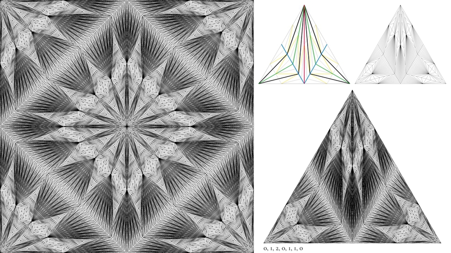
Rather than generating all variations, we will look at a subset. For simplicity and 'symmetric beauty', only subdivisions that are symmetric through the previous division line are considered. These are only the 1st, 5th (center) and last variation on each line in figure 9. Every pair of green lines (3th iteration subdivision line) share one of their endpoints (on the blue line). This approach reduces the number of variations even more, and results in beautiful symmetric images, and straightforward Python code.
In the Python code, the three triangle vertices are referred to with indices 0, 1 and 2. All triangles in one iteration are subdivided in the same way, so this can be defined with a single vertex index for each iteration. A sequence of these vertices can define a subdivision strategy. These vertices can be notated as the shortest non repeating sequence, and whenever we need to make more iterations than the sequence length, we can repeat the sequence. A strategy defined as '0' means: choosing triangle vertex 0 at every iteration. This is exactly the same as strategy '0, 0' and strategy '0, 0, 0' and so on. Alternating between vertices can be strategy '0, 1, 2' (and is the same as strategy '0, 1, 2, 0, 1, 2', but different from '0, 1, 2, 0'.
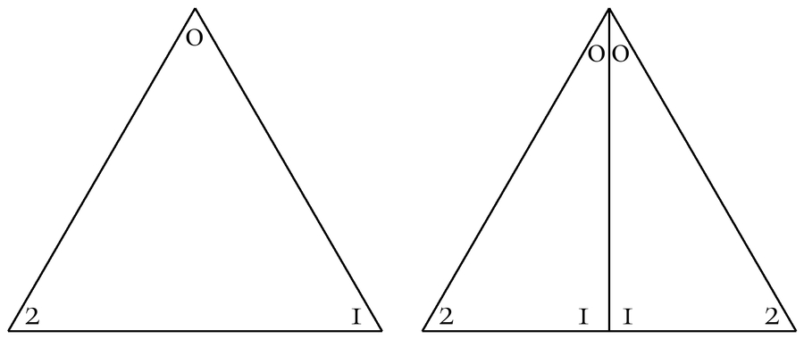
When creating two new triangles at each subdivision, there are several ways to assign vertex indices to those new triangles.
I made the choice to add 0 to the vertex that was chosen to be subdivided, 1 to the new midpoint that was calculated, and 2 to the 'other triangle vertex'.
The two new triangles share vertex 0 and 1 (this is the subdivision line), only vertex 2 is different. This can be seen in figure 10.
Symmetry between the two new triangles is created on purpose.
Note that the triangle indices in the original triangle (on the left) do not matter. Only the 'vertex to subdivide' matters (in this case vertex 0).
So if you would swap indices 0 and 2 on the left triangle, and choose index 2 to subdivide, the result will be exactly the same as the image on the right.
A sequence of 0's means subdividing the same triangle vertex several times (like figure 5 shows).
A sequence of 1's means that the previous midpoint was chosen several times in a row. (see figure 11 and 12)
A sequence of 2's means that the previous subdivision line will be cut in half several times in a row
(because none of the two vertices that define the subdivision line will be chosen, but the 3th vertex).


I chose to add the 'top' triangle vertex first in the code (so it has index 0 in the original triangle).
I want to choose this vertex first for every image I create, so that each image will be symmetrical through this vertical line in the center (the red line in all images).
In Figure 11 you can see what happens if vertex 1 will be chosen over and over again. The result is a grid of triangles.
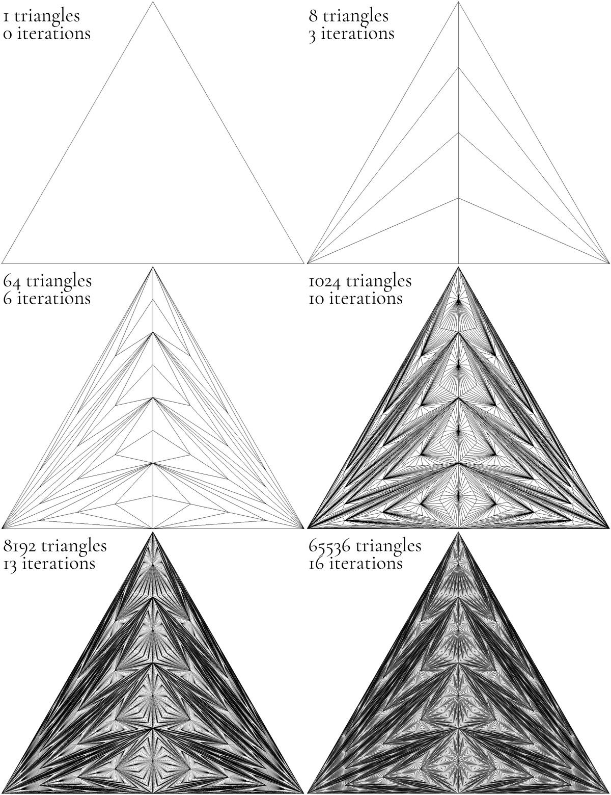
In Figure 12 vertex 1 is chosen three times in a row, and then vertex 0 (the previous vertex again). In the first image are all the division lines for the first 6 iterations are colored differently.
The colors are red, blue, green, black, yellow, and a small grey line for the 6th iteration. The number of lines doubles at every step, so there is 1 red line, but there are in fact 8 different black lines (although some of them seem to line up in this configuration).
The second image has 8 iterations and the last image 13 iterations.
With this logic in place, we could systematically generate a sequence of symmetrical subdivions of this kind.
And for every result, we can assign a name to it (the strategy sequence), so it could be reproduced.
When naively generating all possibilities in increasing sequence length, there will be many repetitions.
All sequences of length 2 will be included in all the sequences of length 4 (and 6, and 8, and so on).
In general, every result of order length n can be found in the results of order length 2 * n, and they could be filtered out.
In the following YouTube video, you can watch more than 3000 of these variations (until sequence length 8). Each strategy sequence is displayed on the bottom right, and could be used in the code below to recreate any image. There is also some additional info in the video description.
The Code
The Python code has been added to my python_shapes repository. Here is a small breakdown.
Triangle vertices are represented as a tuple of two floats, representing x and y coordinates.
A triangle is represented as a list of 3 vertices. Note that the top left of the canvas is (0, 0), and the bottom right has x, y coordinates (width, height).
The triangle vertex with index 0 is the first item in the list of vertices. References to vertices will only be by the position in the list (index 0, 1 or 2).
            triangle = [
               (width / 2, 0),  # vertex 0
               (0, height),  # vertex 1
               (width, height),  # vertex 2
            ]
The midpoint of an edge is calculated by taking the average of the two x coordinates, and the average of the two y coordinates.
            def get_midpoint(point_a, point_b):
                return (
                    (point_a[0] + point_b[0]) / 2,
                    (point_a[1] + point_b[1]) / 2,
                )
To subdivide, we need a function that converts one triangle into two triangles.
This function needs to know the current iteration, and the provided strategy, so it can choose the correct vertex to divide the triangle into two sub triangles.
            def divide(triangle_vertices, iteration, strategy):
                index_to_subdivide = strategy[iteration % len(strategy)]
                subdivide_vertex = triangle_vertices.pop(index_to_subdivide)
                midpoint = get_midpoint(*triangle_vertices)  # midpoint of the remaining two triangle_vertices


                return [
                    [subdivide_vertex, midpoint, triangle_vertices[0]],
                    [subdivide_vertex, midpoint, triangle_vertices[1]],
                ]
The index_to_subdivide takes the correct vertex index from the strategy sequence. This is based on the current iteration,
and when that iteration is larger than the length of the strategy sequence, the modulo operator makes sure it takes the correct index as if the sequence was repeated.
The triangle vertex that will be used to subdivided is called subdivide_vertex and is popped from the list of triangle_vertices. This means that after the pop call, there will be only two vertices left in the triangle_vertices.
The midpoint will be calculated with these two remaining vertices.
The vertices of two new triangles will be returned, in a symmetrical way as shown in figure 10.
With these methods in place, we can generate a subdivided polygon image.
        previous_generation_triangles = [triangle]
        for iteration in range(iterations):
            new_triangles = []
            for triangle in previous_generation_triangles:
                new_triangles += divide(triangle_vertices=triangle, iteration=iteration, strategy=strategy)


            previous_generation_triangles = new_triangles
In the code above, a list of triangles will be constructed. After every iteration, the previous list will be overridden. Since the subdivision is 'complete', all triangle outlines from previous generations are included in the last iteration. At start this list contains one polygon: the starting triangle. After one iteration, it contains two triangles. And so on. When all iterations are done, a list of 2i polygons is constructed. This can be used to draw the polygons.
        for triangle in previous_generation_triangles:
            draw.polygon(xy=triangle, outline=line_color)
I used the Python Imaging Library as you can see in my original code. There is also an even shorter recursive method that produces the same images.
Browser App
There is also a small JavaScript web app that probably works best at a desktop computer or laptop.
It has only been tested in Firefox, but hopefully it works in other browsers too.
You can generate any variation by entering the strategy in the input field, and push one button (or press enter). This works by running JavaScript code in your own browser.
You can also change the 'divisor' (default is 2) to take the midpoint at other places than exactly halfway. The download button will save the result in a .png file.
Conclusion
This way of dividing triangles is a nice showcase of how a sequence of complex looking images can be generated with fairly simple logic and very basic mathematics. There will be a follow up article, since there are more things I would like to share about this.
If you have any corrections, additions, references or comments of any kind, please let me know (info@josvromans.com). I will correct mistakes I made in the math (and in my English writing). There has not been any proof reading or fact checking yet.
As a remark on this process, I can tell that coding my initial triangle division took a short amount of time. Writing this article took me almost two weeks, since it involved a lot of double checking statements, generating images for explanation, and thinking more deeply about what I (and my code) was actually doing. This illustrates in some sense how much there is to write or reason about things that are created by code within minutes. And of course there is so much more to study about this. This is also the reason why I produce a lot of images, but not write many blogs or articles. They take a lot of time, and I find it very difficult to achieve a 'finished' result that I like to share.
If you can think about a more basic triangle subdivision than the one I described in this article, I am happy to discuss that one. The more complex ones are fun to code, but I do not aspire to dive into the details of them. To wrap this up, I will give a few examples of how you can make more complex subdivisions (there are many, many more), and add a few more images of triangle subdivisions.
- - Use two or more different triangle subdivisions in a certain order. Or choose them at random from a set of possible subdivisions.
- - Don't use the same subdivision choice in one iteration for every triangle.
- - There are many 'only triangle' subdivisions possible, think about subdividing into 3 or more triangles. Allow gaps, and allow new triangles to have a different size.
- - subdivide in other n-gons than just triangles. A simple one is to subdivide one triangle into a square
and two triangles, or a square and three triangles. A square can then be easily subdivided into two or four triangles.
- - Allow the subdivision to grow outside the original n-gon. This can generate things (with an outline) similar to Koch's Snowflake, when the growth is limited it the right way.
Alternate between 'subdivide within the original polygon' and 'subdivide and exceed the original polygon dimensions' in some way.
- - Make combinations of the above. This will generate a very large number of variations, and still, it will only be the surface of what is possible.
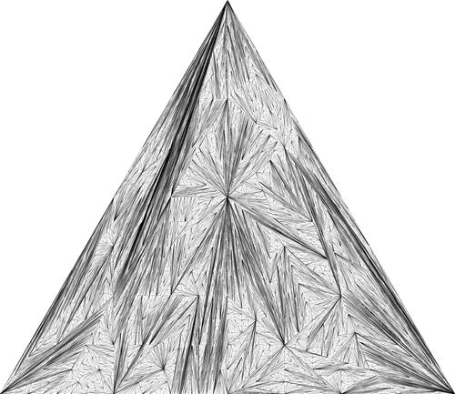 Figure 14: Choosing every vertex at random (imagine analyzing all possibilities if I dropped the symmetry restrictions..)
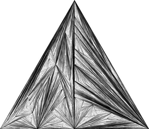
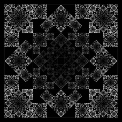 Figure 16: Subdivision with squares and triangles. You can see how this one was created by looking at the steps here.
